Beginner’s Guide: Gridding a Spectral Cube with VisCube#
In this tutorial, we will be using VisCube to grid a spectral cube. For simplicity, this tutorial skips the somewhat arduous process of extracting data from Measurement Sets into memory/numpy (for how to do that using CASA or XRADIO, see here). This tutorial focuses on JUST VisCube’s gridding abilities themselves. For simplicity, we will be doing UV gridding (assuming the array is planar, so no W coordinates, a reasonable assumption for e.g. ALMA).
To demonstrate VisCube’s power, we will be calculating the gridded visibilities AND the associated standard deviations for a spectral cube of galaxy NGC4697!
%load_ext autoreload
%autoreload 2
from viscube import grid_cube_all_stats, load_and_mask, hermitian_augment
import numpy as np
import matplotlib.pyplot as plt
Step 0: Load the numpy file previously extracted from the measurement set#
N.B., this tutorial assumes this numpy file has already been created for you.#
To learn how to create such a numpy file for your measurement sets, see here.
To download this npz file and run this notebook, go here: link to Zenodo
UPDATE: The current file on Zenodo only works with VisCube version <= 0.2.0. An updated version is coming.#
path = "/home/darthbarth/Big_red/NGC4697/cube_extracted_antennae.npz"
data = np.load(path)
freq = data["chan_freq_hz"]
u_raw = data["u"]
v_raw = data["v"]
vis_raw = data["vis"]
weight_raw = data["weight"]
sigma_re_cube = data["sigma_re_cube"]
sigma_im_cube = data["sigma_im_cube"]
mask = data["mask"]
Step 1: Apply the mask#
# Mask + compact
frequencies, u0, v0, vis0, weight0, sigma_re0, sigma_im0 = load_and_mask(
    freq, u_raw, v_raw, vis_raw, weight_raw, sigma_re_cube, sigma_im_cube, mask
)
Step 2: Hermitian Augmentation#
N.B., if you’re working with a continuum dataset (whose shape is (N_vis) rather than (N_freq, N_vis)), you will need to add a [None, N_vis] dimension in order for the gridder to handle things properly (it needs a frequency dimension even if the number of channels is one).
# Hermitian augment (including sigma)
uu, vv, vis_re, vis_imag, wt, sigma_re_aug, sigma_im_aug = hermitian_augment(
    u0, v0, vis0, weight0, sigma_re0, sigma_im0
)
Step 3: Gridding with uncertainty estimation!#
In this example, we use VisCube’s grid_cube_all_stats function, which assumes you want to do UV gridding for a spectral cube and calculate the standard deviation within each grid cell. Other gridding functions in VisCube exist, e.g. grid_cube_all_stats_wbinned, which does UVW gridding instead. For an example of how to use grid_cube_all_stats_wbinned, see this tutorial instead starting from Step 5.
The outputs of grid_cube_all_stats are as follows:
mean_re: the gridded visibilities, real component
mean_im: the gridded visibilities, imaginary component
std_re: standard deviations, per grid cell, of the real components of the gridded visibilities
std_im: standard deviations, per grid cell, of the imaginary components of the gridded visibilities
counts: number of visibilities in each grid cell (can be useful for creating a mask also)
u_edges, v_edges: the edges of the grid in U,V coordinates
# Convert sigma -> inverse variance for fallback branch
eps_sigma = 1e-12
invvar_group_re = 1.0 / np.maximum(sigma_re_aug, eps_sigma)**2
invvar_group_im = 1.0 / np.maximum(sigma_im_aug, eps_sigma)**2
# Grid
std_min_effective = 10
mean_re, mean_im, std_re, std_im, counts, u_edges, v_edges = grid_cube_all_stats(
    frequencies=freq,
    uu=uu,
    vv=vv,
    vis_re=vis_re,
    vis_imag=vis_imag,
    weight=wt,  # your usual weights for mean + empirical std branch
    invvar_group_re=invvar_group_re,
    invvar_group_im=invvar_group_im,
    npix=501,
    window_name="kaiser_bessel",
    window_kwargs={"m": 6},
    std_min_effective=std_min_effective,
)
100%|███████████| 80/80 [02:55<00:00, 2.19s/channel, fallback_pix_im=808, fallback_pix_re=808]
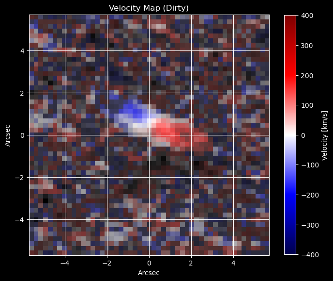
Step 4 (OPTIONAL): Visualize the results as a “dirty image” velocity map using SuperMAGE#
For documentation on how to use SuperMAGE, please see here: https://supermage.readthedocs.io/en/latest/intro.html.
from supermage.utils.plotting import dirty_cube_tool, velocity_map
from supermage.utils.doppler_velocities import create_velocity_grid_stable
fov_arcseconds = 206265*501/(2*461206.80374266725)
num_pixels_uv = 501
arcseconds_per_pixel = fov_arcseconds / num_pixels_uv
freq_path = "/home/darthbarth/Data/ngc_4697/frequencies_correct.npy"
max_freq_index = 74
freq = (np.load(freq_path)/1e9)[:max_freq_index]
systemic_velocity = 1239.9591200072425
velocities_absolute, _ = create_velocity_grid_stable(freq[0], freq[-1], len(freq))
velocities = velocities_absolute.numpy() - systemic_velocity

# Define the region of interest for the cube (pixels 1000 to 1050)
roi_start, roi_end = 225, 276
fov_pixels = roi_end - roi_start
dirty_cube = dirty_cube_tool(mean_re, mean_im, roi_start, roi_end)
extent = (-1*arcseconds_per_pixel*fov_pixels/2, arcseconds_per_pixel*fov_pixels/2, -1*arcseconds_per_pixel*fov_pixels/2, arcseconds_per_pixel*fov_pixels/2)
vel_map = velocity_map(dirty_cube[:, :, :max_freq_index], velocities)
import matplotlib
import matplotlib.pyplot as plt
from matplotlib import animation, rc, colors

plt.style.use('dark_background')
fig, ax1 = plt.subplots(1, 1, figsize = (8, 8))
ax1.set_aspect('equal', adjustable='box')

divnorm=colors.TwoSlopeNorm(vcenter=0., vmin = -400, vmax = 400)
im11 = ax1.imshow(vel_map, cmap = "seismic", norm = divnorm, origin = "lower",  extent=extent)
c_white = matplotlib.colors.colorConverter.to_rgba('white',alpha = 0)
c_black= matplotlib.colors.colorConverter.to_rgba('black',alpha = 1)
cmap_rb = matplotlib.colors.LinearSegmentedColormap.from_list('rb_cmap',[c_black, c_white],256)
im12 = ax1.imshow(np.sum(dirty_cube[:, :, :max_freq_index], axis = 2), cmap = cmap_rb, origin = "lower",  extent=extent)

fig.colorbar(im11, label = "Velocity [km/s]", shrink = 0.8)
ax1.set_xlabel("Arcsec")
ax1.set_ylabel("Arcsec")
ax1.set_title("Velocity Map (Dirty)")
plt.grid()
plt.show()
Step -1: Don’t forget to save your results to disk!#
save_dir1 = "/home/darthbarth/Data/ngc_4697/NGC4697_kaiser_bessel/gridded_visibilities_viscube1.npz"
np.savez(
        save_dir1,
        vis_bin_re   = mean_re,
        vis_bin_imag = mean_im,
        std_bin_re   = std_re,
        std_bin_imag = std_im,
        mask         = counts > 0,
    )